The Elegant Theory of Inflation

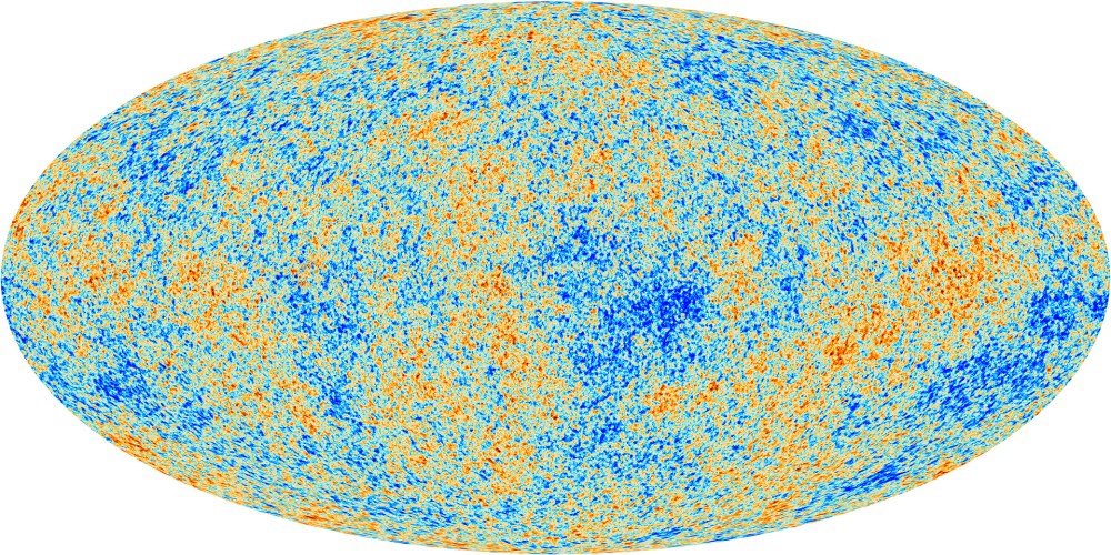
The Cosmic Microwave Background and its anisotropies, as seen by Planck.
Credit: ESA and the Planck Collaboration

Introduction

We live in a 13.8-billion-year-old Universe, today dominated by a cosmological constant (otherwise known as dark energy), something that’s caused the expansion of the Universe to accelerate so much that today, the radius of the observable Universe is over 45 billion light-years (and the actual Universe is far larger than that). The farthest we can see back into our Universe’s past is a mere 380,000 years after the Big Bang, a whisper of the Big Bang left over in the form of radiation producing the Cosmic Microwave Background (CMB), pictured above. The different colors represent little anisotropies, or density fluctuations, in the CMB, which represent the seeds for the formation of the galaxies we see today.

The Early Universe

Today, we live in a Universe that’s composed of ~70% dark energy, ~25% dark matter, and ~5% ordinary matter, or more generally, ~30% matter. A very tiny amount is attributed to radiation today, so small it’s only a tiny fraction of a percent, and can be overlooked in calculations. But this was not the case further back in the Universe’s history. First, and perhaps one of the most bizarre and mind-blowing things, is that the cosmological constant, Λ, which we call dark energy, does not dilute—ie, as the Universe expands, the density of dark energy remains the same. But matter and radiation do dilute, and they dilute at different rates. Radiation dilutes as the scale factor¹ to the negative 4th power, or a^-4, whereas matter dilutes as a^-3. This is a consequence of radiation being relativistic, while matter is non-relativistic.  So, way back when the Universe was younger, matter and radiation were denser, and because the density of dark energy is constant, the Universe was actually dominated by matter and radiation; further back still, radiation was the dominant component of the Universe. The question is, how did all this matter and radiation come about? Did it just pop into existence out of nowhere? Well, the theory of the Big Bang postulates that it all came from a singularity and suddenly, the Universe, all the matter and radiation that come with it, just was (for more details, check out this post from Ethan Siegel). And the theory of the Big Bang describes the Universe astonishingly well, which was confirmed with the discovery of the CMB (as you can read about in the article I linked above).

However, alone, the theory of the Big Bang alone fails to explain some things:

1. Why is the Universe so homogeneous?
2. Why is the Universe flat, as opposed to heavily curved?
3. Why aren’t there any magnetic monopoles?

In the following sections, I’ll discuss these problems in further detail, and you’ll see why conventional Big Bang cosmology cannot account for these problems.

¹The scale factor, a, which is actually a function of time, a(t), is just a parameter that describes the expansion of the Universe with time. By convention, we set the scale factor to 1 today, a(t₀) = 1. The scale factor decreases as we move to the past, and increases as we go forward in time.

The Horizon Problem

Even with the anisotropies in the CMB, this whisper of the Big Bang is pretty darn homogeneous, everywhere the same to an astonishing 1 part in 100,000. Everywhere. The. Same. In a gargantuan Universe. Many points on the CMB are obviously out of causal contact with each other, and yet, they are seemingly in thermal equilibrium with each other. In case you’re wondering what causal contact is, it’s basically this: if two particles, or spaces, can communicate with each other so that they can exchange energy and thermally equilibrate, they are in causal contact; if they are totally out of reach of each other, then they cannot have communicated with each other, and hence are out of causal contact (more on this coming up).

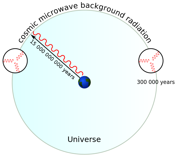
A graphic depicting the CMB some 380,000 years after the Big Bang. The small circles show the extent radiation could reach when the Universe was 380,000 years old, meaning there are plenty of points on the CMB that are causally disconnected.
Credit: Theresa Knott and  Chris 論

Yet, observations show us that all the CMB’s causally disconnected points, separated by distances greater than the particle horizon², are in thermal equilibrium with each other. How can this be? That’s like accepting that a bunch of different apartments across the city have exactly the same furniture set without the tenants having communicated with each other! And by a bunch, I mean 20,000 [1]—that’s how many parts of the CMB are causally disconnected. Sure, you can have a few apartments with exactly the same furniture set. But imagine that 20,000 apartments had the exact same furniture set. Hard to believe these people didn’t talk to each other and say “Hey there’s a really good deal on this furniture set, so let everyone know!”, right? Of course it is. That’s why it’s so startling that observations show the CMB to be 2.725 K everywhere. Conventional Big Bang cosmology cannot explain this. This is the essence of what is known as The Horizon Problem.

²The particle (or comoving) horizon defines the distance a particle can communicate with another. It is its past light cone. If two particles are separated at a distance greater than the particle horizon, the particles could never have communicated with one another because the regions are moving away from each other faster than the speed of light. For example, the observable Universe is defined by our particle horizon, and we can never observe anything beyond it.

The Flatness Problem

We also find the Universe to be incredibly flat. Why is this weird? Well, let’s talk about curvature. There are three possibilities for curvature: a negatively curved Universe (think of a saddle, or a Pringles chip), a positively curved Universe (say, a sphere), and finally, flat (like a sheet of paper). Of course, the Universe has three spatial dimensions (and one time), but our brains can’t think in 3D, so we’re stuck to 2D analogies.

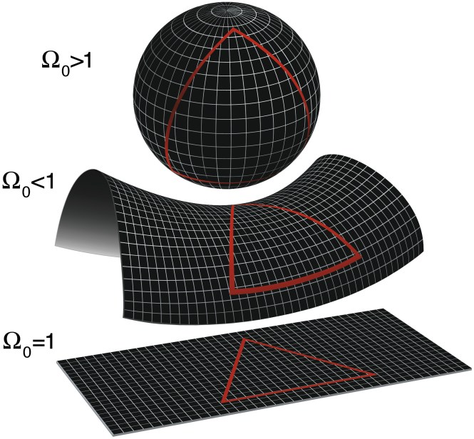
The parameter Ω₀ is known as the density parameter, which tells us the curvature of the Universe. If the energy density of the Universe is greater than the critical density of the Universe, then we get Ω₀ > 1, or a positively curved spacetime. If it is less than the critical density, then
Ω₀ < 1, and space time is negatively curved. But if the energy density is exactly equal to the critical density, Ω₀ = 1, spacetime is flat. Credit: NASA/WMAP Science Team

But, to be flat, the Universe must have (almost) exactly zero curvature, which means the energy density of the Universe must be exactly its critical density. The density parameter, Ω₀ = ρ/ρ_crit, is basically all the components of the Universe added together: the cosmological constant, Ω_Λ, matter, Ω_m, and radiation, Ω_r, which add up to 1 for a flat Universe (i.e. Ω₀ = Ω_Λ + Ω_m + Ω_r). And we find that |1 – Ω₀|= Ω_k ≤ 0.005 today, where Ω_k is the curvature parameter. This means our Universe is really really close to flat. So, why is this a problem? Well, to get to the density parameter we observe today, at the time of Big Bang Nucleosynthesis, when the first nuclei were formed, the curvature parameter had to be 10^-16 (another way to say this is the density parameter could only deviate from 1 by 10^-16); further back to the GUT era, and the curvature parameter needed to be 10^-55; finally, at the Planck time, a mere 5×10^-44 seconds after the Big Bang, we require that the density parameter deviate from 1 by only 10^-61 to get the density parameter as close to 1 as it is today [2]. This, if we rely on conventional Big Bang cosmology. But, why would expansion have not driven the Universe away from flatness? What I’ve described here is The Flatness Problem.

The Monopole Problem

Yet another puzzle is that we don’t find any magnetic monopoles today, but theory tells us that in the extreme heat of the very early Universe, when the strong and electroweak³ forces were unified into one force, monopoles came in copious amounts.

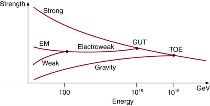
A figure showing the energies at which the forces were united, and the energies at which they became distinct. Source: Lumen Physics

In the above figure, the TOE (the Theory of Everything)⁴ is a point just 10^-43 seconds after the Big Bang, or the Planck time, while temperatures were some 10³² K. That’s far before the time in question. The time in question here is the GUT era, or the Grand Unified Theory. During this time, some 10^-36 seconds after the Big Bang, when the Universe was 10²⁸ K, the strong and electroweak forces were unified. When the temperature, or energy, dropped below the GUT energy of 10¹⁵ GeV, spontaneous symmetry breaking occurred, which gave rise to “topological defects” in the form of magnetic monopoles (other topological defects that could have been created are domain walls and cosmic strings) [3]. The theory of the Big Bang alone tells us there should be lots of magnetic monopoles left over today. Yet, where are they? We have yet to find a single magnetic monopole in nature. This is The Monopole Problem.

³Back when the Universe was some 10¹⁵ K, the electromagnetic force and the weak force were unified into one force: the electroweak force. Eventually the Universe cooled and the two forces became distinct as we see today. More on forces in a future blog post.
⁴The TOE requires unifying gravity with the other forces. It is work that some fields, like string theory, aim to achieve. The Wikipedia article on this provides a good detailed explanation of the TOE.

The Theory of Inflation

As we’ve seen, conventional Big Bang cosmology doesn’t explain how the Universe is so homogeneous and isotropic while 20,000 points are acausal, why the Universe is so flat, and why we don’t see magnetic monopoles today. It would require extreme fine-tuning to work out to what we see today, and we physicists don’t like fine-tuning because it leaves too much up to chance as opposed to explaining how our observations come about and how they make sense, so it’s a big problem to just sweep something like this under the rug and accept that we just so happen to live in these extra-special conditions.

So, physicists did what they do, and came up with a profoundly elegant solution to these problems in theoretical physics—inflation! Alan Guth is the pioneer of this theory, and coined the term. Others, including Andrei Linde, and Paul Steinhardt, did pioneering work on the theory as well.

Inflation is driven by a scalar field (a scalar field just describes a potential energy, similar to, for example, a gravitational potential) known as the “inflaton” that can carry a potential energy that doesn’t dilute (sounds like the cosmological constant, doesn’t it?).

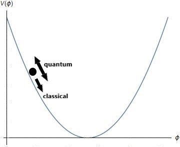
A scalar field in slow-roll inflation, where classically the field rolls down to the minimum, but experiences quantum fluctuations. Plot created in Mathematica (ball and arrows added using Paint 3D)

During a period that lasted some 10^-36 seconds to 10^-33 seconds after the Big Bang, the Universe expanded from submicroscopic to macroscopic with, as stated by my once professor and always fantastic theoretical physicist Matthew Johnson, an e¹⁸⁰ increase in volume (that’s a lot, as in, ~10⁷⁸ times its volume!!) over an unfathomably small period of time. When inflation ends, reheating begins and converts all this potential energy into matter and radiation—that is, the energy that drove inflation is put into reheating the Universe and making radiation and matter, so that it didn’t just pop up out of nowhere, as we are to believe if we rely on conventional Big Bang cosmology alone (this means that the reheating phase is the Big Bang!). And quantum fluctuations translated to the density fluctuations we see in the CMB today, and provided the seeds for dark matter, stars, and galaxies to form in the Universe.

Now that you’ve learned (generally) how inflation works, allow me to show you the brilliance of the inflation solution to the three problems aforementioned, and the exciting implications that come from this theory.

In the coming sections, I have included some mathematical formalisms. I have also indicated where these begin and where they end, so that if you would like to skip over the math, you may do so and still get the concepts. Also, remember there are some footnotes! They might be useful. Without further ado, let’s bring on the physics!

Solution to the Horizon Problem

As we’ve seen, the theory of the Big Bang alone is insufficient to explain the astonishing homogeneity of the Universe. Big Bang cosmology assumes that the Hubble radius⁵ grows monotonically from the Big Bang singularity, meaning the Hubble sphere starts from a point and grows. This means the particle horizons of many points on the CMB are acausal, as shown in the figure below.

In this figure, we see the conventional Big Bang Hubble sphere, our past light cone, and points on the CMB labeled p and q (and their past light cones). Looking at the past light cones, or particle horizons, of p and q, it is quite obvious that the two points could never have communicated. [4]

Then, what if instead of monotonic growth, there is a period where this behavior is inverted, so that the Hubble radius, (aH)^-1, shrinks during inflation?

(A bit of math coming up; skip if you’d like)

The particle horizon can be related to the Hubble radius as follows:

[5]

where . In the conventional Big Bang case, the strong energy condition (SEC)⁶, 1 + 3w > 0 (where w is the pressure P divided by the density ρ), is assumed. This means the contributions to the particle horizon from early times are vanishing, and the dominant contributions come from later times (because we have 1 + 3w in the exponent), which results in acausal points on the CMB. But during inflation, it turns out that the SEC is violated, so that 1 + 3w < 0, which results in the lower limit of the integral dominating the solution, giving us a shrinking Hubble sphere, [4] , which means the particle horizon for the seemingly acausal points coincided, giving them time to thermally equilibrate. The SEC violation and shrinking Hubble sphere relation, along with , are actually conditions for inflation. [6]

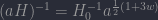
(Math done, continue reading here)

So if the Hubble radius shrinks during inflation, the way the Hubble sphere evolves is sort of “inverted” so that it doesn’t just grow from a point, but rather, shrinks during inflation, and then goes back to its conventional growth. This leads to the Big Bang singularity starting in negative conformal time⁷, so that the seemingly acausal points were once in causal contact, but are seen as acausal on the CMB today.

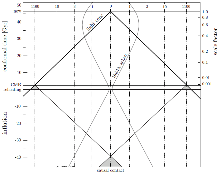
The figure above shows a shrinking Hubble sphere during inflation, which then expands in the Big Bang. The reheating phase becomes the Big Bang. The two points that are acausal on the CMB were causal points during inflation, so that all acausal points were in causal contact. [7]

In summary, with an inflationary period, the acausal points we see on the CMB today were actually far closer prior to inflation—they were causally connected, and thus able to communicate and thermally equilibrate. The Universe expanded exponentially during inflation (recall I said that the Universe grew by ~10⁷⁸ in volume during inflation), so that all these seemingly acausal points did have time to exchange information when they were in causal contact, producing the homogeneous CMB today. For the mathematically inclined reader, refer to my citations at the very end of this article.

⁵The Hubble radius defines the distance at which two regions beyond it cannot talk to each other now—ie, they are acausal now. The particle horizon, however, defines the distance beyond which two regions can never have communicated with each other. This distinction is really important.
⁶The strong energy condition basically states that gravity can’t be repulsive, or that matter always attracts to matter; i.e. pressure cannot be negative.
⁷Conformal time might be better understood as a distance, where the particle horizon is equal to the conformal time passed since the Big Bang, multiplied by the speed of light. It is the time it would take a photon to travel from here to as far into the Universe as we can go, and hence not a physical time: if we froze the expansion of the Universe, it would take a photon ~45 billion light-years to travel there, since the observable Universe is ~45 billion light-years in radius; but the Universe is only 13.8 billion years old. Hence it is better understood as a distance.

Solution to the Flatness Problem

The flatness problem essentially asks: why is the Universe so flat when it could’ve taken on some curvature during its evolution?

(Some math ahead; feel free to skip)

The Friedmann equation, which basically describes the expansion of the Universe, as well as its curvature, is given in the form

where H is the Hubble parameter⁸, a is our friendly scale factor, G is Newton’s Gravitational constant, ρ is the density, and k is the curvature of the Universe (I have set c = 1). To see why it was important for me to bring up some equations, for a flat Universe, k = 0, so that part of the equation disappears, and we’re left with something we can rearrange to form what is called the “critical density”:

And, as I mentioned before, to get to the critical density we have today, we require extreme fine-tuning if we assume the Hubble sphere just grows monotonically, so much that the density parameter, Ω₀=ρ₀/ρ_crit,0, is only allowed to deviate from 1 by very specific and tiny amounts in the early Universe (as described in the section outlining the flatness problem).

Let’s go back to the Friedmann equation, and divide both sides by the Hubble parameter squared, and put it in the following form:

[8]

where here, the density parameter is a function of a, Ω(a) = ρ(a)/ρ_crit(a), and (aH)^-1 is the Hubble radius. Now, if the Hubble radius increases monotonically as assumed in conventional Big Bang cosmology, that causes the curvature k to grow with time, leading to a Universe with a lot of curvature. But, if instead it decreases during inflation, it drives the Universe to flatness instead, solving the problem and yielding a flat Universe today.

Another way to explain this is by noting that during inflation, the Universe expanded exponentially, so that the density parameter was proportional to the negative exponential of the Hubble parameter multiplied by time:

[9]

where H_i is the Hubble parameter during inflation. So then we can express this as

[9]

where t_f describes the time at the end of inflation, t_i describes the time at the beginning of inflation, and N in the exponential is the number of e-foldings⁹ of inflation. Let’s assume there are 100 e-foldings of inflation. Then, regardless of the Universe’s initial curvature (represented on the right side of the above equation), it’s taken down by e^-200, which is ~10^-87, bringing the left side of the equation, |1 – Ω(t_f)|, extremely close to zero, i.e., Ω = 1, and we’re left with a flat Universe.

(Math complete, you can return now!)

What inflation basically does is it acts to drive the Universe to flatness, so that no matter how much curvature you started with, you will end up with a flat Universe. Because of the exponential expansion that the early Universe undergoes due to inflation, we find that after inflation, it flattens the Universe (in Barbara Ryden’s words) “like the proverbial pancake” [9] (ah, this is one of my favorite quotes on this). Take a sphere as an example.

Graphic showing the surface of a sphere as it grows, and ends up appearing flat. Source: Abyss.uoregon.edu

For an ant, a small sphere of radius, say, 1 cm, has a pretty curved surface. Take the sphere and increase its size to 10 cm in radius, and the ant sees the surface as less curved, but still curved. Now let’s increase the size of the sphere to 5 meters in radius. Does it look flat to the ant? It’s certainly more flat than it was, but when the ant walks around, it realizes there’s some curvature. Now, let’s take it to the extreme and make the sphere the size of the Earth (which has a radius of 6731 km). The surface of the sphere is flat to that ant. This is sort of analogous to the Universe being flattened out by inflation. And note that today, since we are bound by our particle horizon, for all we know, we might be seeing a part of the Universe that appears locally flat, but might actually have curvature that we can’t detect because it’s beyond our past light cone! Ah, the Universe is wonderful.

⁸The Hubble parameter, H, is basically a parameter that describes the expansion of the Universe. More precisely, it is determined by multiplying a dimensionless Hubble parameter, h, by 100 km s^-1 Mpc^-1, where h is 0.678 today according to the Planck results, so that H₀ = h × 100  km s^-1 Mpc^-1 = 67.8  km s^-1 Mpc^-1.
⁹When we say e-foldings, it simply means the number that the exponential, e, is raised to. So, if the number of e-foldings is 8, then that means you raise the exponential to the power of 8: e⁸.

Solution to the Monopole Problem

Finally, we come to the monopole problem, which is a particle physics problem that arises from GUT theory. Recall that once the Universe cooled to the point that the strong and electroweak forces became distinct, symmetry breaking occurred, which caused topological defects in the form of monopoles. A familiar topological defect comes from the freezing of water: water as a liquid has its molecules randomly oriented, but when frozen, it doesn’t freeze uniformly, but rather, may have a few layers that begin to freeze separately. Each layer itself will freeze symmetrically, with its molecules aligned, but the other layers will be misaligned with respect to each other. The misalignment of the axes of symmetry creates a two-dimensional topological defect called a domain wall, and you can also get bubbles frozen into the water, which you can take to be the similar to a point-like topological defect, which in this case would be the monopole. And there should be a lot of magnetic monopoles in the Universe, according to GUT theory and using Big Bang cosmology alone.

The number density of monopoles at the time of their creation was about 10⁸² m^-3 [2]. That’s a 1 with 82 zeros behind it, per meter cubed. Turns out they were also very massive. This means they quickly became non-relativistic, meaning they diluted as a^-3, like matter, which would result in monopoles dominating the Universe when it was just 10^-16 seconds old [2]. This is assuming conventional Big Bang cosmology. However, inflation writes the story differently, and explains why we don’t see any in the Universe today.

If monopoles were created before or during inflation, then the exponential expansion of the Universe during inflation would’ve diluted them so much that there would be nearly no chance of detecting one today. Since during inflation, a ∝ e^H_it, the number density of monopoles diluted like n_M ∝ e^-3H_it[10]. Then the 10⁸² m^-3 created diluted to ~10^-49 m^-3 after 100 e-foldings, leaving us with just 15 monopoles per parsec cubed at the end of inflation (where one parsec is equal to 3.26 light-years, and a light-year is equal to 9.46×10¹⁵ meters) [11]. If we take the expansion of the Universe into account from the end of inflation until today, we’re left with just ~10^-61 Mpc^-3[11]… So, yeah, don’t bet on finding a monopole just floating about anytime soon.

Exciting Possibility: Eternal Inflation

Take another look at my plot of the scalar field above. The double arrow indicating quantum fluctuations could actually keep occurring for a larger inflating field, where inflation stops in our Universe, but goes on forever in an eternally inflating field. This is eternal inflation, where quantum fluctuations could birth new universes, including our own. But the field inflates so fast that these “bubble universes” move so far apart that they never come in contact with each other. The eternally inflating field continues to undergo inflation—once inflation begins, it does not stop. Hence, eternal inflation leads to a Multiverse. Alan Guth also argues that nearly all models of inflation lead to eternal inflation, so if inflation is part of our Universe’s history, then our Universe may be one of infinitely many universes.

Could we ever detect a Multiverse? Well, universes could collide with each other. So if our Universe collided with another in the past, it should have left an imprint on the CMB. Finding such an imprint would be evidence that there exists another universe next to our own, which would tell us we’re part of a Multiverse. This is something scientists looked for in the Planck data, but alas, no imprint was found.

There is a way to get evidence for inflation in the early Universe—gravitational waves. But not the ones we’ve detected from black holes—these are B-modes, specifically created by a period of inflation. Briefly, when scientists look for gravitational waves from black holes, they’re looking for the actual gravitational waves produced. From inflation, they are looking for a signal, left in the CMB, that tells us inflation produced gravitational waves (you can read more about the difference between the two in this article by Clara Moskowitz; although the article was written just before the discovery of the first gravitational waves detected by LIGO, it’s still relevant). If the signals of b-modes are ever detected, we can be certain inflation happened, and if inflation is proven to be part of our Universe’s history, Alan Guth would probably assert that eternal inflation just got real. Are you excited about inflation yet?

Citations

1. B. Ryden, Introduction to Cosmology, Chap. 11, Sec. 1, p. 238 (2006).
2. D. Baumann, TASI Lectures on Inflation, p. 25, 2016, arXiv:0608407v1 [astro-ph]
3. B. Ryden, Introduction to Cosmology, Chap. 11, Sec. 3, p. 241 (2006).
4. D. Baumann, Cosmology: Part III Mathematical Tripos, Chap. 2, Sec. 1.2, p. 32.
5. D. Baumann, Cosmology: Part III Mathematical Tripos, Chap. 2, Sec. 1.2, p. 31.
6. D. Baumann, TASI Lectures on Inflation, p. 27, 2016, arXiv:0608407v1 [astro-ph]
7. D. Baumann, Cosmology: Part III Mathematical Tripos, Chap. 2, Sec. 1.2, p. 33.
8. D. Baumann, The Physics of Inflation, Chap. 1, Sec. 3.2, p. 12.
9. B. Ryden, Introduction to Cosmology, Chap. 11, Sec. 4, p. 244 (2006).
10. B. Ryden, Introduction to Cosmology, Chap. 11, Sec. 4, p. 246 (2006).
11. B. Ryden, Introduction to Cosmology, Chap. 11, Sec. 4, p. 247 (2006).

NOTE: All the above references are great for the mathematically inclined reader; for the reader who wants to learn about cosmology, Barbara Ryden’s textbook is a great starter (with a few fantastically humorous footnotes, might I add), but also assumes prior physics knowledge.

Updated June 17, 2017 at 6:27 PM EDT to include definition for (aH)^-1 to explain how SEC affects the evolution of the particle horizon in the case of Big Bang cosmology vs inflation.